See any bugs/typos/confusing explanations? Open a GitHub issue. You can also comment below
★ See also the PDF version of this chapter (better formatting/references) ★
Mathematical Background
- Recall basic mathematical notions such as sets, functions, numbers, logical operators and quantifiers, strings, and graphs.
- Rigorously define Big-\(O\) notation.
- Proofs by induction.
- Practice with reading mathematical definitions, statements, and proofs.
- Transform an intuitive argument into a rigorous proof.
“I found that every number, which may be expressed from one to ten, surpasses the preceding by one unit: afterwards the ten is doubled or tripled … until a hundred; then the hundred is doubled and tripled in the same manner as the units and the tens … and so forth to the utmost limit of numeration.”, Muhammad ibn Mūsā al-Khwārizmī, 820, translation by Fredric Rosen, 1831.
In this chapter we review some of the mathematical concepts that we use in this book. These concepts are typically covered in courses or textbooks on “mathematics for computer science” or “discrete mathematics”; see the “Bibliographical Notes” section (Section 1.9) for several excellent resources on these topics that are freely-available online.
A mathematician’s apology. Some students might wonder why this book contains so much math. The reason is that mathematics is simply a language for modeling concepts in a precise and unambiguous way. In this book we use math to model the concept of computation. For example, we will consider questions such as “is there an efficient algorithm to find the prime factors of a given integer?”. (We will see that this question is particularly interesting, touching on areas as far apart as Internet security and quantum mechanics!) To even phrase such a question, we need to give a precise definition of the notion of an algorithm, and of what it means for an algorithm to be efficient. Also, since there is no empirical experiment to prove the nonexistence of an algorithm, the only way to establish such a result is using a mathematical proof.
This chapter: a reader’s manual
Depending on your background, you can approach this chapter in two different ways:
If you have already taken “discrete mathematics”, “mathematics for computer science” or similar courses, you do not need to read the whole chapter. You can just take a quick look at Section 1.2 to see the main tools we will use, Section 1.7 for our notation and conventions, and then skip ahead to the rest of this book. Alternatively, you can sit back, relax, and read this chapter just to get familiar with our notation, as well as to enjoy (or not) my philosophical musings and attempts at humor.
If your background is less extensive, see Section 1.9 for some resources on these topics. This chapter briefly covers the concepts that we need, but you may find it helpful to see a more in-depth treatment. As usual with math, the best way to get comfortable with this material is to work out exercises on your own.
You might also want to start brushing up on discrete probability, which we’ll use later in this book (see Chapter 18).
A quick overview of mathematical prerequisites
The main mathematical concepts we will use are the following. We just list these notions below, deferring their definitions to the rest of this chapter. If you are familiar with all of these, then you might want to just skip to Section 1.7 to see the full list of notation we use.
Proofs: First and foremost, this book involves a heavy dose of formal mathematical reasoning, which includes mathematical definitions, statements, and proofs.
Sets and set operations: We will use extensively mathematical sets. We use the basic set relations of membership (\(\in\)) and containment (\(\subseteq\)), and set operations, principally union (\(\cup\)), intersection (\(\cap\)), and set difference (\(\setminus\)).
Cartesian product and Kleene star operation: We also use the Cartesian product of two sets \(A\) and \(B\), denoted as \(A \times B\) (that is, \(A \times B\) the set of pairs \((a,b)\) where \(a\in A\) and \(b\in B\)). We denote by \(A^n\) the \(n\) fold Cartesian product (e.g., \(A^3 = A \times A \times A\)) and by \(A^*\) (known as the Kleene star) the union of \(A^n\) for all \(n \in \{0,1,2,\ldots\}\).
Functions: The domain and codomain of a function, properties such as being one-to-one (also known as injective) or onto (also known as surjective) functions, as well as partial functions (that, unlike standard or “total” functions, are not necessarily defined on all elements of their domain).
Logical operations: The operations AND (\(\wedge\)), OR (\(\vee\)), and NOT (\(\neg\)) and the quantifiers “there exists” (\(\exists\)) and “for all” (\(\forall\)).
Basic combinatorics: Notions such as \(\binom{n}{k}\) (the number of \(k\)-sized subsets of a set of size \(n\)).
Graphs: Undirected and directed graphs, connectivity, paths, and cycles.
Big-\(O\) notation: \(O,o,\Omega,\omega,\Theta\) notation for analyzing asymptotic growth of functions.
Discrete probability: We will use probability theory, and specifically probability over finite samples spaces such as tossing \(n\) coins, including notions such as random variables, expectation, and concentration. We will only use probability theory in the second half of this text, and will review it beforehand in Chapter 18. However, probabilistic reasoning is a subtle (and extremely useful!) skill, and it’s always good to start early in acquiring it.
In the rest of this chapter we briefly review the above notions. This is partially to remind the reader and reinforce material that might not be fresh in your mind, and partially to introduce our notation and conventions which might occasionally differ from those you’ve encountered before.
Reading mathematical texts
Mathematicians use jargon for the same reason that it is used in many other professions such as engineering, law, medicine, and others. We want to make terms precise and introduce shorthand for concepts that are frequently reused. Mathematical texts tend to “pack a lot of punch” per sentence, and so the key is to read them slowly and carefully, parsing each symbol at a time.
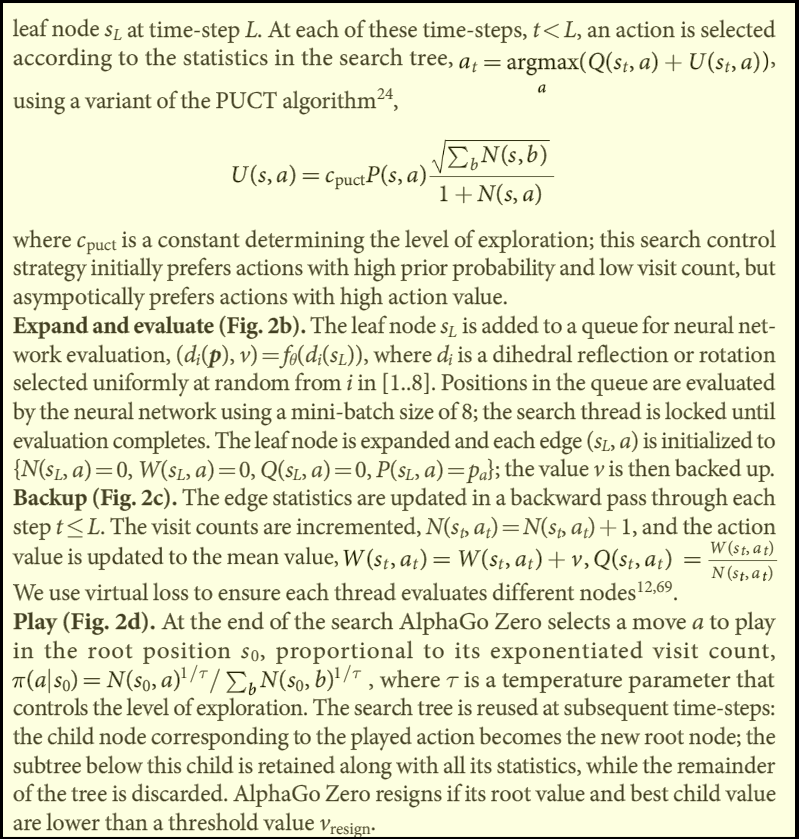
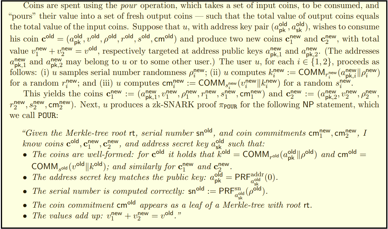
With time and practice you will see that reading mathematical texts becomes easier and jargon is no longer an issue. Moreover, reading mathematical texts is one of the most transferable skills you could take from this book. Our world is changing rapidly, not just in the realm of technology, but also in many other human endeavors, whether it is medicine, economics, law or even culture. Whatever your future aspirations, it is likely that you will encounter texts that use new concepts that you have not seen before (see Figure 1.1 and Figure 1.2 for two recent examples from current “hot areas”). Being able to internalize and then apply new definitions can be hugely important. It is a skill that’s much easier to acquire in the relatively safe and stable context of a mathematical course, where one at least has the guarantee that the concepts are fully specified, and you have access to your teaching staff for questions.
The basic components of a mathematical text are definitions, assertions and proofs.
Definitions
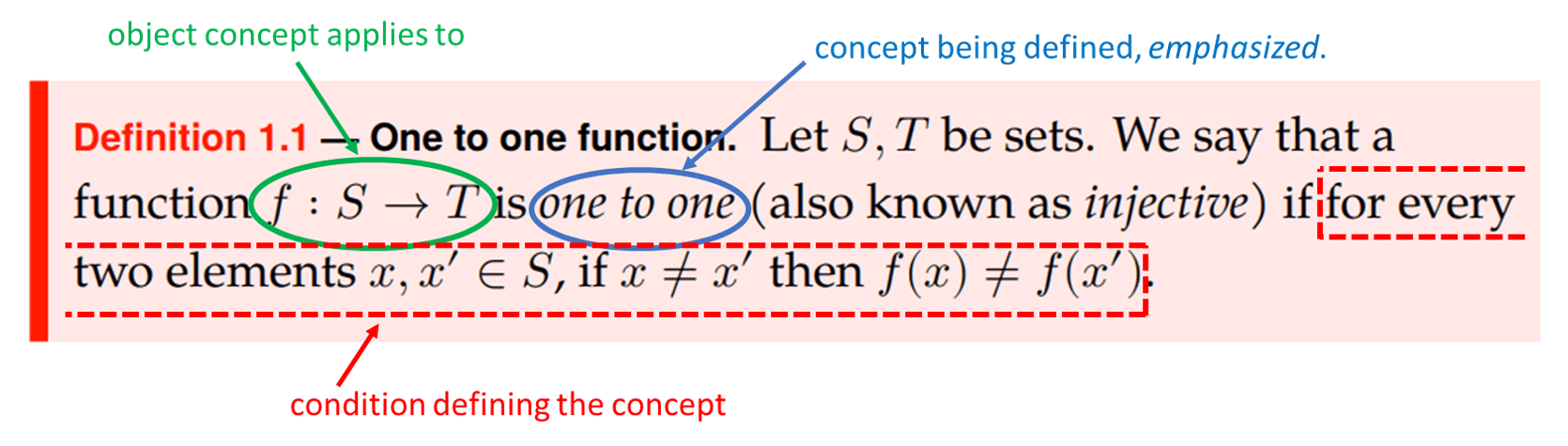
Mathematicians often define new concepts in terms of old concepts. For example, here is a mathematical definition which you may have encountered in the past (and will see again shortly):
Let \(S,T\) be sets. We say that a function \(f:S \rightarrow T\) is one to one (also known as injective) if for every two elements \(x,x' \in S\), if \(x \neq x'\) then \(f(x) \neq f(x')\).
Definition 1.1 captures a simple concept, but even so it uses quite a bit of notation. When reading such a definition, it is often useful to annotate it with a pen as you’re going through it (see Figure 1.3). For example, when you see an identifier such as \(f\), \(S\) or \(x\), make sure that you realize what sort of object it is: is it a set, a function, an element, a number, a gremlin? You might also find it useful to explain the definition in words to a friend (or to yourself).
Assertions: Theorems, lemmas, claims
Theorems, lemmas, claims and the like are true statements about the concepts we defined. Deciding whether to call a particular statement a “Theorem”, a “Lemma” or a “Claim” is a judgement call, and does not make a mathematical difference. All three correspond to statements which were proven to be true. The difference is that a Theorem refers to a significant result that we would want to remember and highlight. A Lemma often refers to a technical result that is not necessarily important in its own right, but that can be often very useful in proving other theorems. A Claim is a “throwaway” statement that we need to use in order to prove some other bigger results, but do not care so much about for its own sake.
Proofs
Mathematical proofs are the arguments we use to demonstrate that our theorems, lemmas, and claims are indeed true. We discuss proofs in Section 1.5 below, but the main point is that the mathematical standard of proof is very high. Unlike in some other realms, in mathematics a proof is an “airtight” argument that demonstrates that the statement is true beyond a shadow of a doubt. Some examples in this section for mathematical proofs are given in Solved Exercise 1.1 and Section 1.6. As mentioned in the preface, as a general rule, it is more important you understand the definitions than the theorems, and it is more important you understand a theorem statement than its proof.
Basic discrete math objects
In this section we quickly review some of the mathematical objects (the “basic data structures” of mathematics, if you will) we use in this book.
Sets
A set is an unordered collection of objects. For example, when we write \(S = \{ 2,4, 7 \}\), we mean that \(S\) denotes the set that contains the numbers \(2\), \(4\), and \(7\). (We use the notation “\(2 \in S\)” to denote that \(2\) is an element of \(S\).) Note that the set \(\{ 2, 4, 7 \}\) and \(\{ 7, 4, 2 \}\) are identical, since they contain the same elements. Also, a set either contains an element or does not contain it – there is no notion of containing it “twice” – and so we could even write the same set \(S\) as \(\{ 2, 2, 4, 7\}\) (though that would be a little weird). The cardinality of a finite set \(S\), denoted by \(|S|\), is the number of elements it contains. (Cardinality can be defined for infinite sets as well; see the sources in Section 1.9.) So, in the example above, \(|S|=3\). A set \(S\) is a subset of a set \(T\), denoted by \(S \subseteq T\), if every element of \(S\) is also an element of \(T\). (We can also describe this by saying that \(T\) is a superset of \(S\).) For example, \(\{2,7\} \subseteq \{ 2,4,7\}\). The set that contains no elements is known as the empty set and it is denoted by \(\emptyset\). If \(A\) is a subset of \(B\) that is not equal to \(B\) we say that \(A\) is a strict subset of \(B\), and denote this by \(A \subsetneq B\).
We can define sets by either listing all their elements or by writing down a rule that they satisfy such as
Of course there is more than one way to write the same set, and often we will use intuitive notation listing a few examples that illustrate the rule. For example, we can also define \(\text{EVEN}\) as
Note that a set can be either finite (such as the set \(\{2,4,7\}\)) or infinite (such as the set \(\text{EVEN}\)). Also, the elements of a set don’t have to be numbers. We can talk about the sets such as the set \(\{a,e,i,o,u \}\) of all the vowels in the English language, or the set \(\{\)New York, Los Angeles, Chicago, Houston, Philadelphia, Phoenix, San Antonio, San Diego, Dallas\(\}\) of all cities in the U.S. with population more than one million per the 2010 census. A set can even have other sets as elements, such as the set \(\{ \emptyset, \{1,2\},\{2,3\},\{1,3\} \}\) of all even-sized subsets of \(\{1,2,3\}\).
Operations on sets: The union of two sets \(S,T\), denoted by \(S \cup T\), is the set that contains all elements that are either in \(S\) or in \(T\). The intersection of \(S\) and \(T\), denoted by \(S \cap T\), is the set of elements that are both in \(S\) and in \(T\). The set difference of \(S\) and \(T\), denoted by \(S \setminus T\) (and in some texts also by \(S-T\)), is the set of elements that are in \(S\) but not in \(T\).
Tuples, lists, strings, sequences: A tuple is an ordered collection of items. For example \((1,5,2,1)\) is a tuple with four elements (also known as a \(4\)-tuple or quadruple). Since order matters, this is not the same tuple as the \(4\)-tuple \((1,1,5,2)\) or the \(3\)-tuple \((1,5,2)\). A \(2\)-tuple is also known as a pair. We use the terms tuples and lists interchangeably. A tuple where every element comes from some finite set \(\Sigma\) (such as \(\{0,1\}\)) is also known as a string. Analogously to sets, we denote the length of a tuple \(T\) by \(|T|\). Just like sets, we can also think of infinite analogues of tuples, such as the ordered collection \((1,4,9,\ldots )\) of all perfect squares. Infinite ordered collections are known as sequences; we might sometimes use the term “infinite sequence” to emphasize this, and use “finite sequence” as a synonym for a tuple. (We can identify a sequence \((a_0,a_1,a_2,\ldots)\) of elements in some set \(S\) with a function \(A:\N \rightarrow S\) (where \(a_n = A(n)\) for every \(n\in \N\)). Similarly, we can identify a \(k\)-tuple \((a_0,\ldots,a_{k-1})\) of elements in \(S\) with a function \(A:[k] \rightarrow S\).)
Cartesian product: If \(S\) and \(T\) are sets, then their Cartesian product, denoted by \(S \times T\), is the set of all ordered pairs \((s,t)\) where \(s\in S\) and \(t\in T\). For example, if \(S = \{1,2,3 \}\) and \(T = \{10,12 \}\), then \(S\times T\) contains the \(6\) elements \((1,10),(2,10),(3,10),(1,12),(2,12),(3,12)\). Similarly if \(S,T,U\) are sets then \(S\times T \times U\) is the set of all ordered triples \((s,t,u)\) where \(s\in S\), \(t\in T\), and \(u\in U\). More generally, for every positive integer \(n\) and sets \(S_0,\ldots,S_{n-1}\), we denote by \(S_0 \times S_1 \times \cdots \times S_{n-1}\) the set of ordered \(n\)-tuples \((s_0,\ldots,s_{n-1})\) where \(s_i\in S_i\) for every \(i \in \{0,\ldots, n-1\}\). For every set \(S\), we denote the set \(S\times S\) by \(S^2\), \(S\times S\times S\) by \(S^3\), \(S\times S\times S \times S\) by \(S^4\), and so on and so forth.
Special sets
There are several sets that we will use in this book time and again. The set
We will also occasionally use the set \(\Z=\{\ldots,-2,-1,0,+1,+2,\ldots \}\) of (negative and non-negative) integers,1 as well as the set \(\R\) of real numbers. (This is the set that includes not just the integers, but also fractional and irrational numbers; e.g., \(\R\) contains numbers such as \(+0.5\), \(-\pi\), etc.) We denote by \(\R_+\) the set \(\{ x\in \R : x > 0 \}\) of positive real numbers. This set is sometimes also denoted as \((0,\infty)\).
Strings: Another set we will use time and again is
We will write the string \((x_0,x_1,\ldots,x_{n-1})\) as simply \(x_0x_1\cdots x_{n-1}\). For example,
For every string \(x\in \{0,1\}^n\) and \(i\in [n]\), we write \(x_i\) for the \(i^{th}\) element of \(x\).
We will also often talk about the set of binary strings of all lengths, which is
Another way to write this set is as
The set \(\{0,1\}^*\) includes the “string of length \(0\)” or “the empty string”, which we will denote by \(\ensuremath{\text{\texttt{""}}}\). (In using this notation we follow the convention of many programming languages. Other texts sometimes use \(\epsilon\) or \(\lambda\) to denote the empty string.)
Generalizing the star operation: For every set \(\Sigma\), we define
Concatenation: The concatenation of two strings \(x\in \Sigma^n\) and \(y\in \Sigma^m\) is the \((n+m)\)-length string \(xy\) obtained by writing \(y\) after \(x\). That is, if \(x \in \{0,1\}^n\) and \(y\in \{0,1\}^m\), then \(xy\) is equal to the string \(z\in \{0,1\}^{n+m}\) such that for \(i\in [n]\), \(z_i=x_i\) and for \(i\in \{n,\ldots,n+m-1\}\), \(z_i = y_{i-n}\).
Functions
If \(S\) and \(T\) are non-empty sets, a function \(F\) mapping \(S\) to \(T\), denoted by \(F:S \rightarrow T\), associates with every element \(x\in S\) an element \(F(x)\in T\). The set \(S\) is known as the domain of \(F\) and the set \(T\) is known as the codomain of \(F\). The image of a function \(F\) is the set \(\{ F(x) \;|\; x\in S\}\) which is the subset of \(F\)’s codomain consisting of all output elements that are mapped from some input. (Some texts use range to denote the image of a function, while other texts use range to denote the codomain of a function. Hence we will avoid using the term “range” altogether.) As in the case of sets, we can write a function either by listing the table of all the values it gives for elements in \(S\) or by using a rule. For example if \(S = \{0,1,2,3,4,5,6,7,8,9 \}\) and \(T = \{0,1 \}\), then the table below defines a function \(F: S \rightarrow T\). Note that this function is the same as the function defined by the rule \(F(x)= (x \mod 2)\).2
| Input | Output |
|---|---|
| 0 | 0 |
| 1 | 1 |
| 2 | 0 |
| 3 | 1 |
| 4 | 0 |
| 5 | 1 |
| 6 | 0 |
| 7 | 1 |
| 8 | 0 |
| 9 | 1 |
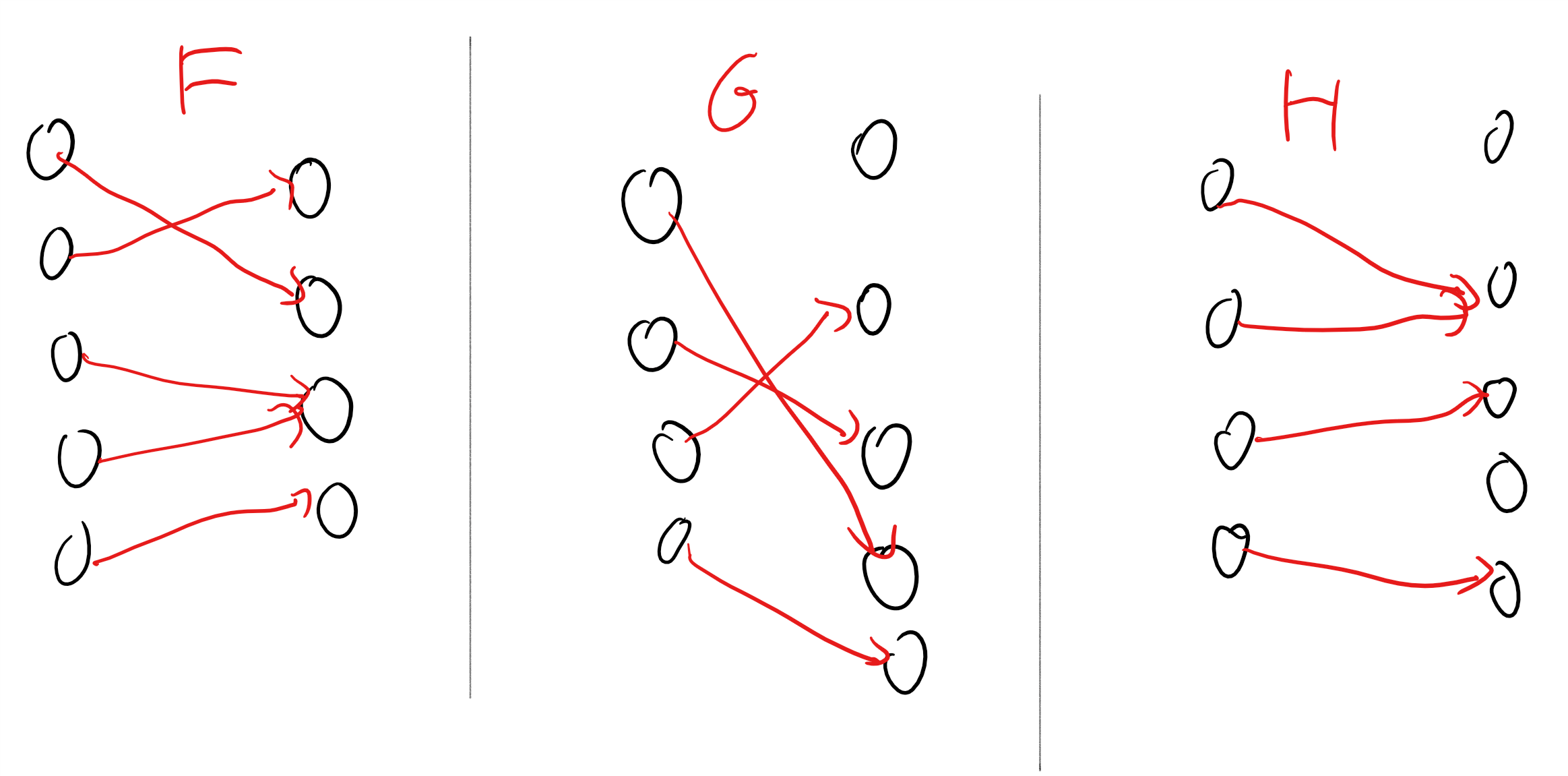
If \(F:S \rightarrow T\) satisfies that \(F(x)\neq F(y)\) for all \(x \neq y\) then we say that \(F\) is one-to-one (Definition 1.1, also known as an injective function or simply an injection). If \(F\) satisfies that for every \(y\in T\) there is some \(x\in S\) such that \(F(x)=y\) then we say that \(F\) is onto (also known as a surjective function or simply a surjection). A function that is both one-to-one and onto is known as a bijective function or simply a bijection. A bijection from a set \(S\) to itself is also known as a permutation of \(S\). If \(F:S \rightarrow T\) is a bijection then for every \(y\in T\) there is a unique \(x\in S\) such that \(F(x)=y\). We denote this value \(x\) by \(F^{-1}(y)\). Note that \(F^{-1}\) is itself a bijection from \(T\) to \(S\) (can you see why?).
Giving a bijection between two sets is often a good way to show they have the same size. In fact, the standard mathematical definition of the notion that “\(S\) and \(T\) have the same cardinality” is that there exists a bijection \(f:S \rightarrow T\). Further, the cardinality of a set \(S\) is defined to be \(n\) if there is a bijection from \(S\) to the set \(\{0,\ldots,n-1\}\). As we will see later in this book, this is a definition that generalizes to defining the cardinality of infinite sets.
Partial functions: We will sometimes be interested in partial functions from \(S\) to \(T\). A partial function is allowed to be undefined on some subset of \(S\). That is, if \(F\) is a partial function from \(S\) to \(T\), then for every \(s\in S\), either there is (as in the case of standard functions) an element \(F(s)\) in \(T\), or \(F(s)\) is undefined. For example, the partial function \(F(x)= \sqrt{x}\) is only defined on non-negative real numbers. When we want to distinguish between partial functions and standard (i.e., non-partial) functions, we will call the latter total functions. When we say “function” without any qualifier then we mean a total function.
The notion of partial functions is a strict generalization of functions, and so every function is a partial function, but not every partial function is a function. (That is, for every non-empty \(S\) and \(T\), the set of partial functions from \(S\) to \(T\) is a proper superset of the set of total functions from \(S\) to \(T\).) When we want to emphasize that a function \(f\) from \(A\) to \(B\) might not be total, we will write \(f: A \rightarrow_p B\). We can think of a partial function \(F\) from \(S\) to \(T\) also as a total function from \(S\) to \(T \cup \{ \bot \}\) where \(\bot\) is a special “failure symbol”. So, instead of saying that \(F\) is undefined at \(x\), we can say that \(F(x)=\bot\).
Basic facts about functions: Verifying that you can prove the following results is an excellent way to brush up on functions:
If \(F:S \rightarrow T\) and \(G:T \rightarrow U\) are one-to-one functions, then their composition \(H:S \rightarrow U\) defined as \(H(s)=G(F(s))\) is also one to one.
If \(F:S \rightarrow T\) is one to one, then there exists an onto function \(G:T \rightarrow S\) such that \(G(F(s))=s\) for every \(s\in S\).
If \(G:T \rightarrow S\) is onto then there exists a one-to-one function \(F:S \rightarrow T\) such that \(G(F(s))=s\) for every \(s\in S\).
If \(S\) and \(T\) are non-empty finite sets then the following conditions are equivalent to one another: (a) \(|S| \leq |T|\), (b) there is a one-to-one function \(F:S \rightarrow T\), and (c) there is an onto function \(G:T \rightarrow S\). These equivalences are in fact true even for infinite \(S\) and \(T\). For infinite sets the condition (b) (or equivalently, (c)) is the commonly accepted definition for \(|S| \leq |T|\).
You can find the proofs of these results in many discrete math texts, including for example, Section 4.5 in the Lehman-Leighton-Meyer notes. However, I strongly suggest you try to prove them on your own, or at least convince yourself that they are true by proving special cases of those for small sizes (e.g., \(|S|=3,|T|=4,|U|=5\)).
Let us prove one of these facts as an example:
If \(S,T\) are non-empty sets and \(F:S \rightarrow T\) is one to one, then there exists an onto function \(G:T \rightarrow S\) such that \(G(F(s))=s\) for every \(s\in S\).
Choose some \(s_0 \in S\). We will define the function \(G:T \rightarrow S\) as follows: for every \(t\in T\), if there is some \(s\in S\) such that \(F(s)=t\) then set \(G(t)=s\) (the choice of \(s\) is well defined since by the one-to-one property of \(F\), there cannot be two distinct \(s,s'\) that both map to \(t\)). Otherwise, set \(G(t)=s_0\). Now for every \(s\in S\), by the definition of \(G\), if \(t=F(s)\) then \(G(t)=G(F(s))=s\). Moreover, this also shows that \(G\) is onto, since it means that for every \(s\in S\) there is some \(t\), namely \(t=F(s)\), such that \(G(t)=s\).
Graphs
Graphs are ubiquitous in Computer Science, and many other fields as well. They are used to model a variety of data types including social networks, scheduling constraints, road networks, deep neural nets, gene interactions, correlations between observations, and a great many more. Formal definitions of several kinds of graphs are given next, but if you have not seen graphs before in a course, I urge you to read up on them in one of the sources mentioned in Section 1.9.
Graphs come in two basic flavors: undirected and directed.3
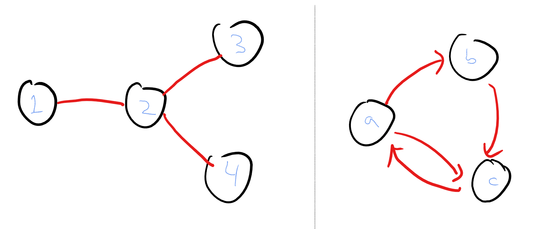
An undirected graph \(G = (V,E)\) consists of a set \(V\) of vertices and a set \(E\) of edges. Every edge is a size two subset of \(V\). We say that two vertices \(u,v \in V\) are neighbors, if the edge \(\{u,v\}\) is in \(E\).
Given this definition, we can define several other properties of graphs and their vertices. We define the degree of \(u\) to be the number of neighbors \(u\) has. A path in the graph is a tuple \((u_0,\ldots,u_k) \in V^{k+1}\), for some \(k>0\) such that \(u_{i+1}\) is a neighbor of \(u_i\) for every \(i\in [k]\). A simple path is a path \((u_0,\ldots,u_{k-1})\) where all the \(u_i\)’s are distinct. A cycle is a path \((u_0,\ldots,u_k)\) where \(u_0=u_{k}\). We say that two vertices \(u,v\in V\) are connected if either \(u=v\) or there is a path from \((u_0,\ldots,u_k)\) where \(u_0=u\) and \(u_k=v\). We say that the graph \(G\) is connected if every pair of vertices in it is connected.
Here are some basic facts about undirected graphs. We give some informal arguments below, but leave the full proofs as exercises (the proofs can be found in many of the resources listed in Section 1.9).
In any undirected graph \(G=(V,E)\), the sum of the degrees of all vertices is equal to twice the number of edges.
Lemma 1.4 can be shown by seeing that every edge \(\{ u,v\}\) contributes twice to the sum of the degrees (once for \(u\) and the second time for \(v\)).
The connectivity relation is transitive, in the sense that if \(u\) is connected to \(v\), and \(v\) is connected to \(w\), then \(u\) is connected to \(w\).
Lemma 1.5 can be shown by simply attaching a path of the form \((u,u_1,u_2,\ldots,u_{k-1},v)\) to a path of the form \((v,u'_1,\ldots,u'_{k'-1},w)\) to obtain the path \((u,u_1,\ldots,u_{k-1},v,u'_1,\ldots,u'_{k'-1},w)\) that connects \(u\) to \(w\).
For every undirected graph \(G=(V,E)\) and connected pair \(u,v\), the shortest path from \(u\) to \(v\) is simple. In particular, for every connected pair there exists a simple path that connects them.
Lemma 1.6 can be shown by “shortcutting” any non-simple path from \(u\) to \(v\) where the same vertex \(w\) appears twice to remove it (see Figure 1.6). It is a good exercise to transforming this intuitive reasoning to a formal proof:
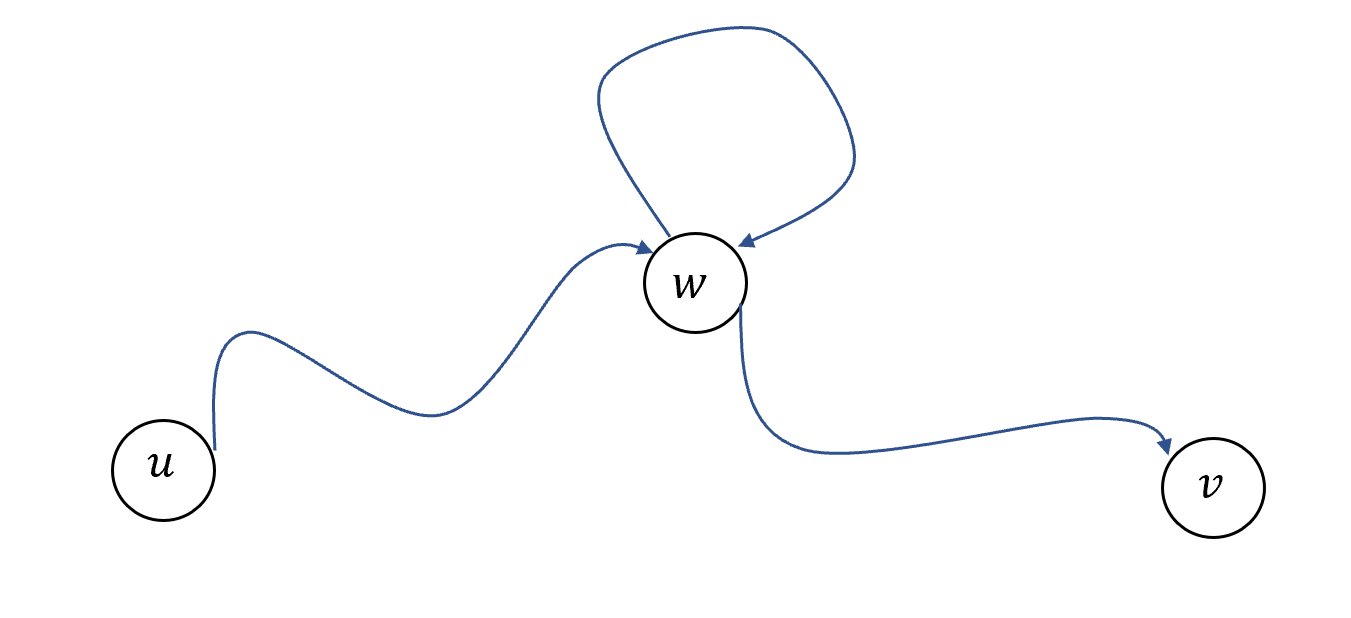
Prove Lemma 1.6
The proof follows the idea illustrated in Figure 1.6. One complication is that there can be more than one vertex that is visited twice by a path, and so “shortcutting” might not necessarily result in a simple path; we deal with this by looking at a shortest path between \(u\) and \(v\). Details follow.
Let \(G=(V,E)\) be a graph and \(u\) and \(v\) in \(V\) be two connected vertices in \(G\). We will prove that there is a simple path between \(u\) and \(v\). Let \(k\) be the shortest length of a path between \(u\) and \(v\) and let \(P=(u_0,u_1,u_2,\ldots,u_{k-1},u_k)\) be a \(k\)-length path from \(u\) to \(v\) (there can be more than one such path: if so we just choose one of them). (That is \(u_0=u\), \(u_k=v\), and \((u_\ell,u_{\ell+1})\in E\) for all \(\ell \in [k]\).) We claim that \(P\) is simple. Indeed, suppose otherwise that there is some vertex \(w\) that occurs twice in the path: \(w = u_i\) and \(w=u_j\) for some \(i<j\). Then we can “shortcut” the path \(P\) by considering the path \(P' = (u_0,u_1,\ldots,u_{i-1},w,u_{j+1},\ldots,u_k)\) obtained by taking the first \(i\) vertices of \(P\) (from \(u_0=0\) to the first occurrence of \(w\)) and the last \(k-j\) ones (from the vertex \(u_{j+1}\) following the second occurrence of \(w\) to \(u_k=v\)). The path \(P'\) is a valid path between \(u\) and \(v\) since every consecutive pair of vertices in it is connected by an edge (in particular, since \(w=u_i=u_j\), both \((u_{i-1},w)\) and \((w,u_{j+1})\) are edges in \(E\)), but since the length of \(P'\) is \(k-(j-i)<k\), this contradicts the minimality of \(P\).
Solved Exercise 1.1 is a good example of the process of finding a proof. You start by ensuring you understand what the statement means, and then come up with an informal argument why it should be true. You then transform the informal argument into a rigorous proof. This proof need not be very long or overly formal, but should clearly establish why the conclusion of the statement follows from its assumptions.
The concepts of degrees and connectivity extend naturally to directed graphs, defined as follows.
A directed graph \(G=(V,E)\) consists of a set \(V\) and a set \(E \subseteq V\times V\) of ordered pairs of \(V\). We sometimes denote the edge \((u,v)\) also as \(u \rightarrow v\). If the edge \(u \rightarrow v\) is present in the graph then we say that \(v\) is an out-neighbor of \(u\) and \(u\) is an in-neighbor of \(v\).
A directed graph might contain both \(u \rightarrow v\) and \(v \rightarrow u\) in which case \(u\) will be both an in-neighbor and an out-neighbor of \(v\) and vice versa. The in-degree of \(u\) is the number of in-neighbors it has, and the out-degree of \(v\) is the number of out-neighbors it has. A path in the graph is a tuple \((u_0,\ldots,u_k) \in V^{k+1}\), for some \(k>0\) such that \(u_{i+1}\) is an out-neighbor of \(u_i\) for every \(i\in [k]\). As in the undirected case, a simple path is a path \((u_0,\ldots,u_{k-1})\) where all the \(u_i\)’s are distinct and a cycle is a path \((u_0,\ldots,u_k)\) where \(u_0=u_{k}\). One type of directed graphs we often care about is directed acyclic graphs or DAGs, which, as their name implies, are directed graphs without any cycles:
We say that \(G=(V,E)\) is a directed acyclic graph (DAG) if it is a directed graph and there does not exist a list of vertices \(u_0,u_1,\ldots,u_k \in V\) such that \(u_0=u_k\) and for every \(i\in [k]\), the edge \(u_i \rightarrow u_{i+1}\) is in \(E\).
The lemmas we mentioned above have analogs for directed graphs. We again leave the proofs (which are essentially identical to their undirected analogs) as exercises.
In any directed graph \(G=(V,E)\), the sum of the in-degrees is equal to the sum of the out-degrees, which is equal to the number of edges.
In any directed graph \(G\), if there is a path from \(u\) to \(v\) and a path from \(v\) to \(w\), then there is a path from \(u\) to \(w\).
For every directed graph \(G=(V,E)\) and a pair \(u,v\) such that there is a path from \(u\) to \(v\), the shortest path from \(u\) to \(v\) is simple.
For some applications we will consider labeled graphs, where the vertices or edges have associated labels (which can be numbers, strings, or members of some other set). We can think of such a graph as having an associated (possibly partial) labelling function \(L:V \cup E \rightarrow \mathcal{L}\), where \(\mathcal{L}\) is the set of potential labels. However we will typically not refer explicitly to this labeling function and simply say things such as “vertex \(v\) has the label \(\alpha\)”.
Logic operators and quantifiers
If \(P\) and \(Q\) are some statements that can be true or false, then \(P\) AND \(Q\) (denoted as \(P \wedge Q\)) is a statement that is true if and only if both \(P\) and \(Q\) are true, and \(P\) OR \(Q\) (denoted as \(P \vee Q\)) is a statement that is true if and only if either \(P\) or \(Q\) is true. The negation of \(P\), denoted as \(\neg P\) or \(\overline{P}\), is true if and only if \(P\) is false.
Suppose that \(P(x)\) is a statement that depends on some parameter \(x\) (also sometimes known as an unbound variable) in the sense that for every instantiation of \(x\) with a value from some set \(S\), \(P(x)\) is either true or false. For example, \(x>7\) is a statement that is not a priori true or false, but becomes true or false whenever we instantiate \(x\) with some real number. We denote by \(\forall_{x\in S} P(x)\) the statement that is true if and only if \(P(x)\) is true for every \(x\in S\).4 We denote by \(\exists_{x\in S} P(x)\) the statement that is true if and only if there exists some \(x\in S\) such that \(P(x)\) is true.
For example, the following is a formalization of the true statement that there exists a natural number \(n\) larger than \(100\) that is not divisible by \(3\):
“For sufficiently large \(n\).” One expression that we will see come up time and again in this book is the claim that some statement \(P(n)\) is true “for sufficiently large \(n\)”. What this means is that there exists an integer \(N_0\) such that \(P(n)\) is true for every \(n>N_0\). We can formalize this as \(\exists_{N_0\in \N} \forall_{n>N_0} P(n)\).
Quantifiers for summations and products
The following shorthands for summing up or taking products of several numbers are often convenient. If \(S = \{s_0,\ldots,s_{n-1} \}\) is a finite set and \(f:S \rightarrow \R\) is a function, then we write \(\sum_{x\in S} f(x)\) as shorthand for
and \(\prod_{x\in S} f(x)\) as shorthand for
For example, the sum of the squares of all numbers from \(1\) to \(100\) can be written as
Since summing up over intervals of integers is so common, there is a special notation for it. For every two integers, \(a \leq b\), \(\sum_{i=a}^b f(i)\) denotes \(\sum_{i\in S} f(i)\) where \(S =\{ x\in \Z : a \leq x \leq b \}\). Hence, we can write the sum Equation 1.1 as
Parsing formulas: bound and free variables
In mathematics, as in coding, we often have symbolic “variables” or “parameters”. It is important to be able to understand, given some formula, whether a given variable is bound or free in this formula. For example, in the following statement \(n\) is free but \(a\) and \(b\) are bound by the \(\exists\) quantifier:
Since \(n\) is free, it can be set to any value, and the truth of the statement Equation 1.2 depends on the value of \(n\). For example, if \(n=8\) then Equation 1.2 is true, but for \(n=11\) it is false. (Can you see why?)
The same issue appears when parsing code. For example, in the following snippet from the C programming language
for (int i=0 ; i<n ; i=i+1) {
    printf("*");
}
the variable i is bound within the for block but the variable n is free.
The main property of bound variables is that we can rename them (as long as the new name doesn’t conflict with another used variable) without changing the meaning of the statement. Thus for example the statement
is equivalent to Equation 1.2 in the sense that it is true for exactly the same set of \(n\)’s.
Similarly, the code
for (int j=0 ; j<n ; j=j+1) {
    printf("*");
}
produces the same result as the code above that used i instead of j.
Mathematical notation has a lot of similarities with programming language, and for the same reasons. Both are formalisms meant to convey complex concepts in a precise way. However, there are some cultural differences. In programming languages, we often try to use meaningful variable names such as NumberOfVertices while in math we often use short identifiers such as \(n\). Part of it might have to do with the tradition of mathematical proofs as being handwritten and verbally presented, as opposed to typed up and compiled. Another reason is if the wrong variable name is used in a proof, at worst it causes confusion to readers; when the wrong variable name is used in a program, planes might crash, patients might die, and rockets could explode.
One consequence of that is that in mathematics we often end up reusing identifiers, and also “run out” of letters and hence use Greek letters too, as well as distinguish between small and capital letters and different font faces. Similarly, mathematical notation tends to use quite a lot of “overloading”, using operators such as \(+\) for a great variety of objects (e.g., real numbers, matrices, finite field elements, etc..), and assuming that the meaning can be inferred from the context.
Both fields have a notion of “types”, and in math we often try to reserve certain letters for variables of a particular type. For example, variables such as \(i,j,k,\ell,m,n\) will often denote integers, and \(\epsilon\) will often denote a small positive real number (see Section 1.7 for more on these conventions). When reading or writing mathematical texts, we usually don’t have the advantage of a “compiler” that will check type safety for us. Hence it is important to keep track of the type of each variable, and see that the operations that are performed on it “make sense”.
Kun’s book (Kun, 2018) contains an extensive discussion on the similarities and differences between the cultures of mathematics and programming.
Asymptotics and Big-\(O\) notation
“\(\log\log\log n\) has been proved to go to infinity, but has never been observed to do so.”, Anonymous, quoted by Carl Pomerance (2000)
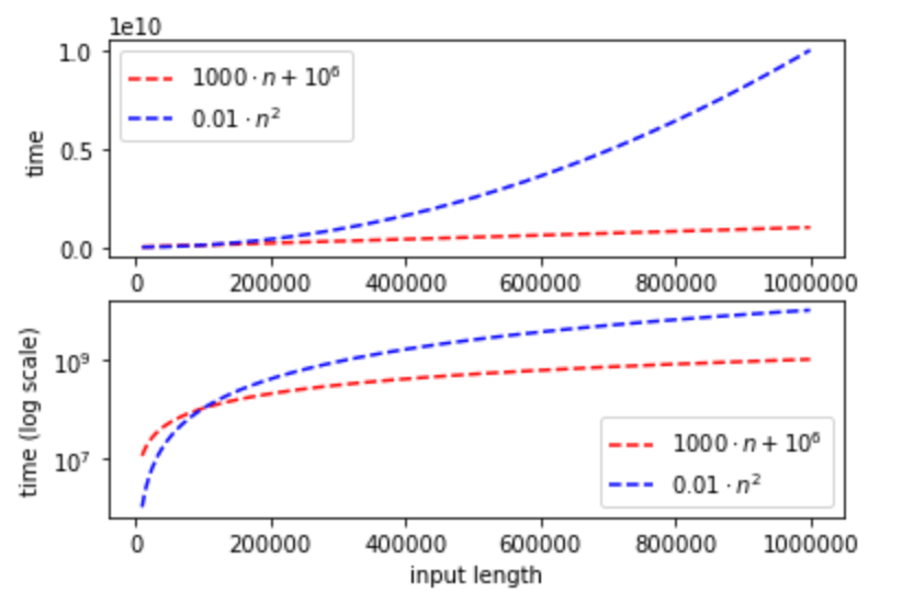
It is often very cumbersome to describe precisely quantities such as running time and is also not needed, since we are typically mostly interested in the “higher order terms”. That is, we want to understand the scaling behavior of the quantity as the input variable grows. For example, as far as running time goes, the difference between an \(n^5\)-time algorithm and an \(n^2\)-time one is much more significant than the difference between a \(100n^2 + 10n\) time algorithm and a \(10n^2\) time algorithm. For this purpose, \(O\)-notation is extremely useful as a way to “declutter” our text and focus our attention on what really matters. For example, using \(O\)-notation, we can say that both \(100n^2 + 10n\) and \(10n^2\) are simply \(\Theta(n^2)\) (which informally means “the same up to constant factors”), while \(n^2 = o(n^5)\) (which informally means that \(n^2\) is “much smaller than” \(n^5\)).
Generally (though still informally), if \(F,G\) are two functions mapping natural numbers to non-negative reals, then “\(F=O(G)\)” means that \(F(n) \leq G(n)\) if we don’t care about constant factors, while “\(F=o(G)\)” means that \(F\) is much smaller than \(G\), in the sense that no matter by what constant factor we multiply \(F\), if we take \(n\) to be large enough then \(G\) will be bigger (for this reason, sometimes \(F=o(G)\) is written as \(F \ll G\)). We will write \(F= \Theta(G)\) if \(F=O(G)\) and \(G=O(F)\), which one can think of as saying that \(F\) is the same as \(G\) if we don’t care about constant factors. More formally, we define Big-\(O\) notation as follows:
Let \(\R_+= \{ x\in \R \;|\; x>0\}\) be the set of positive real numbers. For two functions \(F,G: \N \rightarrow \R_+\), we say that \(F=O(G)\) if there exist numbers \(a,N_0 \in \N\) such that \(F(n) \leq a\cdot G(n)\) for every \(n>N_0\). We say that \(F= \Theta(G)\) if \(F=O(G)\) and \(G=O(F)\). We say that \(F=\Omega(G)\) if \(G=O(F)\).
We say that \(F =o(G)\) if for every \(\epsilon>0\) there is some \(N_0\) such that \(F(n) <\epsilon G(n)\) for every \(n>N_0\). We say that \(F =\omega(G)\) if \(G=o(F)\).
It’s often convenient to use “anonymous functions” in the context of \(O\)-notation. For example, when we write a statement such as \(F(n) = O(n^3)\), we mean that \(F=O(G)\) where \(G\) is the function defined by \(G(n)=n^3\). Chapter 7 in Jim Apsnes’ notes on discrete math provides a good summary of \(O\) notation; see also this tutorial for a gentler and more programmer-oriented introduction.
\(O\) is not equality. Using the equality sign for \(O\)-notation is extremely common, but is somewhat of a misnomer, since a statement such as \(F = O(G)\) really means that \(F\) is in the set \(\{ G' : \exists_{N,c} \text{ s.t. } \forall_{n>N} G'(n) \leq c G(n) \}\). If anything, it makes more sense to use inequalities and write \(F \leq O(G)\) and \(F \geq \Omega(G)\), reserving equality for \(F = \Theta(G)\), and so we will sometimes use this notation too, but since the equality notation is quite firmly entrenched we often stick to it as well. (Some texts write \(F \in O(G)\) instead of \(F = O(G)\), but we will not use this notation.) Despite the misleading equality sign, you should remember that a statement such as \(F = O(G)\) means that \(F\) is “at most” \(G\) in some rough sense when we ignore constants, and a statement such as \(F = \Omega(G)\) means that \(F\) is “at least” \(G\) in the same rough sense.
Some “rules of thumb” for Big-\(O\) notation
There are some simple heuristics that can help when trying to compare two functions \(F\) and \(G\):
Multiplicative constants don’t matter in \(O\)-notation, and so if \(F(n)=O(G(n))\) then \(100F(n)=O(G(n))\).
When adding two functions, we only care about the larger one. For example, for the purpose of \(O\)-notation, \(n^3+100n^2\) is the same as \(n^3\), and in general in any polynomial, we only care about the larger exponent.
For every two constants \(a,b>0\), \(n^a = O(n^b)\) if and only if \(a \leq b\), and \(n^a = o(n^b)\) if and only if \(a<b\). For example, combining the two observations above, \(100n^2 + 10n + 100 = o(n^3)\).
Polynomial is always smaller than exponential: \(n^a = o(2^{n^\epsilon})\) for every two constants \(a>0\) and \(\epsilon>0\) even if \(\epsilon\) is much smaller than \(a\). For example, \(100n^{100} = o(2^{\sqrt{n}})\).
Similarly, logarithmic is always smaller than polynomial: \((\log n)^a\) (which we write as \(\log^a n\)) is \(o(n^\epsilon)\) for every two constants \(a,\epsilon>0\). For example, combining the observations above, \(100n^2 \log^{100} n = o(n^3)\).
While Big-\(O\) notation is often used to analyze running time of algorithms, this is by no means the only application. We can use \(O\) notation to bound asymptotic relations between any functions mapping integers to positive numbers. It can be used regardless of whether these functions are a measure of running time, memory usage, or any other quantity that may have nothing to do with computation. Here is one example which is unrelated to this book (and hence one that you can feel free to skip): one way to state the Riemann Hypothesis (one of the most famous open questions in mathematics) is that it corresponds to the conjecture that the number of primes between \(0\) and \(n\) is equal to \(\int_2^n \tfrac{1}{\ln x} dx\) up to an additive error of magnitude at most \(O(\sqrt{n}\log n)\).
Proofs
Many people think of mathematical proofs as a sequence of logical deductions that starts from some axioms and ultimately arrives at a conclusion. In fact, some dictionaries define proofs that way. This is not entirely wrong, but at its essence, a mathematical proof of a statement X is simply an argument that convinces the reader that X is true beyond a shadow of a doubt.
To produce such a proof you need to:
Understand precisely what X means.
Convince yourself that X is true.
Write your reasoning down in plain, precise and concise English (using formulas or notation only when they help clarity).
In many cases, the first part is the most important one. Understanding what a statement means is oftentimes more than halfway towards understanding why it is true. In the third part, to convince the reader beyond a shadow of a doubt, we will often want to break down the reasoning to “basic steps”, where each basic step is simple enough to be “self-evident”. The combination of all steps yields the desired statement.
Proofs and programs
There is a great deal of similarity between the process of writing proofs and that of writing programs, and both require a similar set of skills. Writing a program involves:
Understanding what is the task we want the program to achieve.
Convincing yourself that the task can be achieved by a computer, perhaps by planning on a whiteboard or notepad how you will break it up into simpler tasks.
Converting this plan into code that a compiler or interpreter can understand, by breaking up each task into a sequence of the basic operations of some programming language.
In programs as in proofs, step 1 is often the most important one. A key difference is that the reader for proofs is a human being and the reader for programs is a computer. (This difference is eroding with time as more proofs are being written in a machine verifiable form; moreover, to ensure correctness and maintainability of programs, it is important that they can be read and understood by humans.) Thus our emphasis is on readability and having a clear logical flow for our proof (which is not a bad idea for programs as well). When writing a proof, you should think of your audience as an intelligent but highly skeptical and somewhat petty reader, that will “call foul” at every step that is not well justified.
Proof writing style
A mathematical proof is a piece of writing, but it is a specific genre of writing with certain conventions and preferred styles. As in any writing, practice makes perfect, and it is also important to revise your drafts for clarity.
In a proof for the statement \(X\), all the text between the words “Proof:” and “QED” should be focused on establishing that \(X\) is true. Digressions, examples, or ruminations should be kept outside these two words, so they do not confuse the reader. The proof should have a clear logical flow in the sense that every sentence or equation in it should have some purpose and it should be crystal-clear to the reader what this purpose is. When you write a proof, for every equation or sentence you include, ask yourself:
Is this sentence or equation stating that some statement is true?
If so, does this statement follow from the previous steps, or are we going to establish it in the next step?
What is the role of this sentence or equation? Is it one step towards proving the original statement, or is it a step towards proving some intermediate claim that you have stated before?
Finally, would the answers to questions 1-3 be clear to the reader? If not, then you should reorder, rephrase, or add explanations.
Some helpful resources on mathematical writing include this handout by Lee, this handout by Hutching, as well as several of the excellent handouts in Stanford’s CS 103 class.
Patterns in proofs
“If it was so, it might be; and if it were so, it would be; but as it isn’t, it ain’t. That’s logic.”, Lewis Carroll, Through the looking-glass.
Just like in programming, there are several common patterns of proofs that occur time and again. Here are some examples:
Proofs by contradiction: One way to prove that \(X\) is true is to show that if \(X\) was false it would result in a contradiction. Such proofs often start with a sentence such as “Suppose, towards a contradiction, that \(X\) is false” and end with deriving some contradiction (such as a violation of one of the assumptions in the theorem statement). Here is an example:
There are no natural numbers \(a,b\) such that \(\sqrt{2} = \tfrac{a}{b}\).
Suppose, towards a contradiction that this is false, and so let \(a\in \N\) be the smallest number such that there exists some \(b\in\N\) satisfying \(\sqrt{2}=\tfrac{a}{b}\). Squaring this equation we get that \(2=a^2/b^2\) or \(a^2=2b^2\) \((*)\). But this means that \(a^2\) is even, and since the product of two odd numbers is odd, it means that \(a\) is even as well, or in other words, \(a = 2a'\) for some \(a' \in \N\). Yet plugging this into \((*)\) shows that \(4a'^2 = 2b^2\) which means \(b^2 = 2a'^2\) is an even number as well. By the same considerations as above we get that \(b\) is even and hence \(a/2\) and \(b/2\) are two natural numbers satisfying \(\tfrac{a/2}{b/2}=\sqrt{2}\), contradicting the minimality of \(a\).
Proofs of a universal statement: Often we want to prove a statement \(X\) of the form “Every object of type \(O\) has property \(P\).” Such proofs often start with a sentence such as “Let \(o\) be an object of type \(O\)” and end by showing that \(o\) has the property \(P\). Here is a simple example:
For every natural number \(n\in N\), either \(n\) or \(n+1\) is even.
Let \(n\in N\) be some number. If \(n/2\) is a whole number then we are done, since then \(n=2(n/2)\) and hence it is even. Otherwise, \(n/2+1/2\) is a whole number, and hence \(2(n/2+1/2)=n+1\) is even.
Proofs of an implication: Another common case is that the statement \(X\) has the form “\(A\) implies \(B\)”. Such proofs often start with a sentence such as “Assume that \(A\) is true” and end with a derivation of \(B\) from \(A\). Here is a simple example:
If \(b^2 \geq 4ac\) then there is a solution to the quadratic equation \(ax^2 + bx + c =0\).
Suppose that \(b^2 \geq 4ac\). Then \(d = b^2 - 4ac\) is a non-negative number and hence it has a square root \(s\). Thus \(x = (-b+s)/(2a)\) satisfies
Rearranging the terms of Equation 1.4 we get
Proofs of equivalence: If a statement has the form “\(A\) if and only if \(B\)” (often shortened as “\(A\) iff \(B\)”) then we need to prove both that \(A\) implies \(B\) and that \(B\) implies \(A\). We call the implication that \(A\) implies \(B\) the “only if” direction, and the implication that \(B\) implies \(A\) the “if” direction.
Proofs by combining intermediate claims: When a proof is more complex, it is often helpful to break it apart into several steps. That is, to prove the statement \(X\), we might first prove statements \(X_1\),\(X_2\), and \(X_3\) and then prove that \(X_1 \wedge X_2 \wedge X_3\) implies \(X\). (Recall that \(\wedge\) denotes the logical AND operator.)
Proofs by case distinction: This is a special case of the above, where to prove a statement \(X\) we split into several cases \(C_1,\ldots,C_k\), and prove that (a) the cases are exhaustive, in the sense that one of the cases \(C_i\) must happen and (b) go one by one and prove that each one of the cases \(C_i\) implies the result \(X\) that we are after.
Proofs by induction: We discuss induction and give an example in Section 1.6.1 below. We can think of such proofs as a variant of the above, where we have an unbounded number of intermediate claims \(X_0,X_1,X_2,\ldots,X_k\), and we prove that \(X_0\) is true, as well as that \(X_0\) implies \(X_1\), and that \(X_0 \wedge X_1\) implies \(X_2\), and so on and so forth. The website for CMU course 15-251 contains a useful handout on potential pitfalls when making proofs by induction.
“Without loss of generality (w.l.o.g)”: This term can be initially quite confusing. It is essentially a way to simplify proofs by case distinctions. The idea is that if Case 1 is equal to Case 2 up to a change of variables or a similar transformation, then the proof of Case 1 will also imply the proof of Case 2. It is always a statement that should be viewed with suspicion. Whenever you see it in a proof, ask yourself if you understand why the assumption made is truly without loss of generality, and when you use it, try to see if the use is indeed justified. When writing a proof, sometimes it might be easiest to simply repeat the proof of the second case (adding a remark that the proof is very similar to the first one).
Mathematical proofs are ultimately written in English prose. The well-known computer scientist Leslie Lamport argues that this is a problem, and proofs should be written in a more formal and rigorous way. In his manuscript he proposes an approach for structured hierarchical proofs, that have the following form:
A proof for a statement of the form “If \(A\) then \(B\)” is a sequence of numbered claims, starting with the assumption that \(A\) is true, and ending with the claim that \(B\) is true.
Every claim is followed by a proof showing how it is derived from the previous assumptions or claims.
The proof for each claim is itself a sequence of subclaims.
The advantage of Lamport’s format is that the role that every sentence in the proof plays is very clear. It is also much easier to transform such proofs into machine-checkable forms. The disadvantage is that such proofs can be tedious to read and write, with less differentiation between the important parts of the arguments versus the more routine ones.
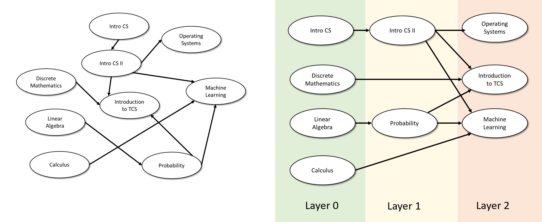
Extended example: Topological Sorting
In this section we will prove the following: every directed acyclic graph (DAG, see Definition 1.9) can be arranged in layers so that for all directed edges \(u \rightarrow v\), the layer of \(v\) is larger than the layer of \(u\). This result is known as topological sorting and is used in many applications, including task scheduling, build systems, software package management, spreadsheet cell calculations, and many others (see Figure 1.8). In fact, we will also use it ourselves later on in this book.
We start with the following definition. A layering of a directed graph is a way to assign for every vertex \(v\) a natural number (corresponding to its layer), such that \(v\)’s in-neighbors are in lower-numbered layers than \(v\), and \(v\)’s out-neighbors are in higher-numbered layers. The formal definition is as follows:
Let \(G=(V,E)\) be a directed graph. A layering of \(G\) is a function \(f:V \rightarrow \N\) such that for every edge \(u \rightarrow v\) of \(G\), \(f(u) < f(v)\).
In this section we prove that a directed graph is acyclic if and only if it has a valid layering.
Let \(G\) be a directed graph. Then \(G\) is acyclic if and only if there exists a layering \(f\) of \(G\).
To prove such a theorem, we need to first understand what it means. Since it is an “if and only if” statement, Theorem 1.22 corresponds to two statements:
For every directed graph \(G\), if \(G\) is acyclic then it has a layering.
For every directed graph \(G\), if \(G\) has a layering, then it is acyclic.
To prove Theorem 1.22 we need to prove both Lemma 1.23 and Lemma 1.24. Lemma 1.24 is actually not that hard to prove. Intuitively, if \(G\) contains a cycle, then it cannot be the case that all edges on the cycle increase in layer number, since if we travel along the cycle at some point we must come back to the place we started from. The formal proof is as follows:
Let \(G=(V,E)\) be a directed graph and let \(f:V \rightarrow \N\) be a layering of \(G\) as per Definition 1.21 . Suppose, towards a contradiction, that \(G\) is not acyclic, and hence there exists some cycle \(u_0,u_1,\ldots,u_k\) such that \(u_0=u_k\) and for every \(i\in [k]\) the edge \(u_i \rightarrow u_{i+1}\) is present in \(G\). Since \(f\) is a layering, for every \(i \in [k]\), \(f(u_i) < f(u_{i+1})\), which means that
Lemma 1.23 corresponds to the more difficult (and useful) direction. To prove it, we need to show how, given an arbitrary DAG \(G\), we can come up with a layering of the vertices of \(G\) so that all edges “go up”.
If you have not seen the proof of this theorem before (or don’t remember it), this would be an excellent point to pause and try to prove it yourself. One way to do it would be to describe an algorithm that given as input a directed acyclic graph \(G\) on \(n\) vertices and \(n-2\) or fewer edges, constructs an array \(F\) of length \(n\) such that for every edge \(u \rightarrow v\) in the graph \(F[u] < F[v]\).
Mathematical induction
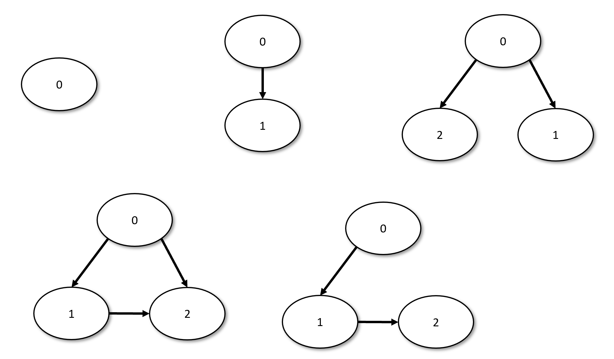
There are several ways to prove Lemma 1.23. One approach to do is to start by proving it for small graphs, such as graphs with 1, 2 or 3 vertices (see Figure 1.9, for which we can check all the cases, and then try to extend the proof for larger graphs). The technical term for this proof approach is proof by induction.
Induction is simply an application of the self-evident Modus Ponens rule that says that if
(a) \(P\) is true
and
(b) \(P\) implies \(Q\)
then \(Q\) is true.
In the setting of proofs by induction we typically have a statement \(Q(k)\) that is parameterized by some integer \(k\), and we prove that (a) \(Q(0)\) is true, and (b) For every \(k>0\), if \(Q(0),\ldots,Q(k-1)\) are all true then \(Q(k)\) is true. (Usually proving (b) is the hard part, though there are examples where the “base case” (a) is quite subtle.) By applying Modus Ponens, we can deduce from (a) and (b) that \(Q(1)\) is true. Once we did so, since we now know that both \(Q(0)\) and \(Q(1)\) are true, then we can use this and (b) to deduce (again using Modus Ponens) that \(Q(2)\) is true. We can repeat the same reasoning again and again to obtain that \(Q(k)\) is true for every \(k\). The statement (a) is called the “base case”, while (b) is called the “inductive step”. The assumption in (b) that \(Q(i)\) holds for \(i<k\) is called the “inductive hypothesis”. (The form of induction described here is sometimes called “strong induction” as opposed to “weak induction” where we replace (b) by the statement (b’) that if \(Q(k-1)\) is true then \(Q(k)\) is true; weak induction can be thought of as the special case of strong induction where we don’t use the assumption that \(Q(0),\ldots,Q(k-2)\) are true.)
Proofs by induction are closely related to algorithms by recursion. In both cases we reduce solving a larger problem to solving a smaller instance of itself. In a recursive algorithm to solve some problem P on an input of length \(k\) we ask ourselves “what if someone handed me a way to solve P on instances smaller than \(k\)?”. In an inductive proof to prove a statement Q parameterized by a number \(k\), we ask ourselves “what if I already knew that \(Q(k')\) is true for \(k'<k\)?”. Both induction and recursion are crucial concepts for this course and Computer Science at large (and even other areas of inquiry, including not just mathematics but other sciences as well). Both can be confusing at first, but with time and practice they become clearer. For more on proofs by induction and recursion, you might find the following Stanford CS 103 handout, this MIT 6.00 lecture or this excerpt of the Lehman-Leighton book useful.
Proving the result by induction
There are several ways to prove Lemma 1.23 by induction. We will use induction on the number \(n\) of vertices, and so we will define the statement \(Q(n)\) as follows:
\(Q(n)\) is “For every DAG \(G=(V,E)\) with \(n\) vertices, there is a layering of \(G\).”
The statement for \(Q(0)\) (where the graph contains no vertices) is trivial. Thus it will suffice to prove the following: for every \(n>0\), if \(Q(n-1)\) is true then \(Q(n)\) is true.
To do so, we need to somehow find a way, given a graph \(G\) of \(n\) vertices, to reduce the task of finding a layering for \(G\) into the task of finding a layering for some other graph \(G'\) of \(n-1\) vertices. The idea is that we will find a source of \(G\): a vertex \(v\) that has no in-neighbors. We can then assign to \(v\) the layer \(0\), and layer the remaining vertices using the inductive hypothesis in layers \(1,2,\ldots\).
The above is the intuition behind the proof of Lemma 1.23, but when writing the formal proof below, we use the benefit of hindsight, and try to streamline what was a messy journey into a linear and easy-to-follow flow of logic that starts with the word “Proof:” and ends with “QED” or the symbol \(\blacksquare\).5 Discussions, examples and digressions can be very insightful, but we keep them outside the space delimited between these two words, where (as described by this excellent handout) “every sentence must be load-bearing”. Just like we do in programming, we can break the proof into little “subroutines” or “functions” (known as lemmas or claims in math language), which will be smaller statements that help us prove the main result. However, the proof should be structured in a way that ensures that it is always crystal-clear to the reader in what stage we are of the proof. The reader should be able to tell what the role of every sentence is in the proof and which part it belongs to. We now present the formal proof of Lemma 1.23.
Let \(G=(V,E)\) be a DAG and \(n=|V|\) be the number of its vertices. We prove the lemma by induction on \(n\). The base case is \(n=0\) where there are no vertices, and so the statement is trivially true.6 For the case of \(n>0\), we make the inductive hypothesis that every DAG \(G'\) of at most \(n-1\) vertices has a layering.
We make the following claim:
Claim: \(G\) must contain a vertex \(v\) of in-degree zero.
Proof of Claim: Suppose otherwise that every vertex \(v\in V\) has an in-neighbor. Let \(v_0\) be some vertex of \(G\), let \(v_1\) be an in-neighbor of \(v_0\), \(v_2\) be an in-neighbor of \(v_1\), and continue in this way for \(n\) steps until we construct a list \(v_0,v_1,\ldots,v_n\) such that for every \(i\in [n]\), \(v_{i+1}\) is an in-neighbor of \(v_i\), or in other words the edge \(v_{i+1} \rightarrow v_i\) is present in the graph. Since there are only \(n\) vertices in this graph, one of the \(n+1\) vertices in this sequence must repeat itself, and so there exists \(i<j\) such that \(v_i=v_j\). But then the sequence \(v_j \rightarrow v_{j-1} \rightarrow \cdots \rightarrow v_i\) is a cycle in \(G\), contradicting our assumption that it is acyclic. (QED Claim)
Given the claim, we can let \(v_0\) be some vertex of in-degree zero in \(G\), and let \(G'\) be the graph obtained by removing \(v_0\) from \(G\). \(G'\) has \(n-1\) vertices and hence per the inductive hypothesis has a layering \(f':(V \setminus \{v_0\}) \rightarrow \N\). We define \(f:V \rightarrow \N\) as follows:
We claim that \(f\) is a valid layering, namely that for every edge \(u \rightarrow v\), \(f(u) < f(v)\). To prove this, we split into cases:
Case 1: \(u \neq v_0\), \(v \neq v_0\). In this case the edge \(u \rightarrow v\) exists in the graph \(G'\) and hence by the inductive hypothesis \(f'(u) < f'(v)\) which implies that \(f'(u)+1 < f'(v)+1\).
Case 2: \(u=v_0\), \(v \neq v_0\). In this case \(f(u)=0\) and \(f(v) = f'(v)+1>0\).
Case 3: \(u \neq v_0\), \(v=v_0\). This case can’t happen since \(v_0\) does not have in-neighbors.
Case 4: \(u=v_0, v=v_0\). This case again can’t happen since it means that \(v_0\) is its own-neighbor — it is involved in a self loop which is a form cycle that is disallowed in an acyclic graph.
Thus, \(f\) is a valid layering for \(G\) which completes the proof.
Reading a proof is no less of an important skill than producing one. In fact, just like understanding code, it is a highly non-trivial skill in itself. Therefore I strongly suggest that you re-read the above proof, asking yourself at every sentence whether the assumption it makes is justified, and whether this sentence truly demonstrates what it purports to achieve. Another good habit is to ask yourself when reading a proof for every variable you encounter (such as \(u\), \(i\), \(G'\), \(f'\), etc. in the above proof) the following questions: (1) What type of variable is it? Is it a number? a graph? a vertex? a function? and (2) What do we know about it? Is it an arbitrary member of the set? Have we shown some facts about it?, and (3) What are we trying to show about it?.
Minimality and uniqueness
Theorem 1.22 guarantees that for every DAG \(G=(V,E)\) there exists some layering \(f:V \rightarrow \N\) but this layering is not necessarily unique. For example, if \(f:V \rightarrow \N\) is a valid layering of the graph then so is the function \(f'\) defined as \(f'(v) = 2\cdot f(v)\). However, it turns out that the minimal layering is unique. A minimal layering is one where every vertex is given the smallest layer number possible. We now formally define minimality and state the uniqueness theorem:
Let \(G=(V,E)\) be a DAG. We say that a layering \(f:V \rightarrow \N\) is minimal if for every vertex \(v \in V\), if \(v\) has no in-neighbors then \(f(v)=0\) and if \(v\) has in-neighbors then there exists an in-neighbor \(u\) of \(v\) such that \(f(u) = f(v)-1\).
For every layering \(f,g:V \rightarrow \N\) of \(G\), if both \(f\) and \(g\) are minimal then \(f=g\).
The definition of minimality in Theorem 1.26 implies that for every vertex \(v \in V\), we cannot move it to a lower layer without making the layering invalid. If \(v\) is a source (i.e., has in-degree zero) then a minimal layering \(f\) must put it in layer \(0\), and for every other \(v\), if \(f(v)=i\), then we cannot modify this to set \(f(v) \leq i-1\) since there is an-neighbor \(u\) of \(v\) satisfying \(f(u)=i-1\). What Theorem 1.26 says is that a minimal layering \(f\) is unique in the sense that every other minimal layering is equal to \(f\).
The idea is to prove the theorem by induction on the layers. If \(f\) and \(g\) are minimal then they must agree on the source vertices, since both \(f\) and \(g\) should assign these vertices to layer \(0\). We can then show that if \(f\) and \(g\) agree up to layer \(i-1\), then the minimality property implies that they need to agree in layer \(i\) as well. In the actual proof we use a small trick to save on writing. Rather than proving the statement that \(f=g\) (or in other words that \(f(v)=g(v)\) for every \(v\in V\)), we prove the weaker statement that \(f(v) \leq g(v)\) for every \(v\in V\). (This is a weaker statement since the condition that \(f(v)\) is lesser or equal than to \(g(v)\) is implied by the condition that \(f(v)\) is equal to \(g(v)\).) However, since \(f\) and \(g\) are just labels we give to two minimal layerings, by simply changing the names “\(f\)” and “\(g\)” the same proof also shows that \(g(v) \leq f(v)\) for every \(v\in V\) and hence that \(f=g\).
Let \(G=(V,E)\) be a DAG and \(f,g:V \rightarrow \N\) be two minimal valid layerings of \(G\). We will prove that for every \(v \in V\), \(f(v) \leq g(v)\). Since we didn’t assume anything about \(f,g\) except their minimality, the same proof will imply that for every \(v\in V\), \(g(v) \leq f(v)\) and hence that \(f(v)=g(v)\) for every \(v\in V\), which is what we needed to show.
We will prove that \(f(v) \leq g(v)\) for every \(v \in V\) by induction on \(i = f(v)\). The case \(i=0\) is immediate: since in this case \(f(v)=0\), \(g(v)\) must be at least \(f(v)\). For the case \(i>0\), by the minimality of \(f\), if \(f(v)=i\) then there must exist some in-neighbor \(u\) of \(v\) such that \(f(u) = i-1\). By the induction hypothesis we get that \(g(u) \geq i-1\), and since \(g\) is a valid layering it must hold that \(g(v) > g(u)\) which means that \(g(v) \geq i = f(v)\).
The proof of Theorem 1.26 is fully rigorous, but is written in a somewhat terse manner. Make sure that you read through it and understand why this is indeed an airtight proof of the Theorem’s statement.
This book: notation and conventions
Most of the notation we use in this book is standard and is used in most mathematical texts. The main points where we diverge are:
We index the natural numbers \(\N\) starting with \(0\) (though many other texts, especially in computer science, do the same).
We also index the set \([n]\) starting with \(0\), and hence define it as \(\{0,\ldots,n-1\}\). In other texts it is often defined as \(\{1,\ldots, n \}\). Similarly, we index our strings starting with \(0\), and hence a string \(x\in \{0,1\}^n\) is written as \(x_0x_1\cdots x_{n-1}\).
If \(n\) is a natural number then \(1^n\) does not equal the number \(1\) but rather this is the length \(n\) string \(11\cdots 1\) (that is a string of \(n\) ones). Similarly, \(0^n\) refers to the length \(n\) string \(00 \cdots 0\).
Partial functions are functions that are not necessarily defined on all inputs. When we write \(f:A \rightarrow B\) this means that \(f\) is a total function unless we say otherwise. When we want to emphasize that \(f\) can be a partial function, we will sometimes write \(f: A \rightarrow_p B\).
As we will see later on in the course, we will mostly describe our computational problems in terms of computing a Boolean function \(f: \{0,1\}^* \rightarrow \{0,1\}\). In contrast, many other textbooks refer to the same task as deciding a language \(L \subseteq \{0,1\}^*\). These two viewpoints are equivalent, since for every set \(L\subseteq \{0,1\}^*\) there is a corresponding function \(F\) such that \(F(x)=1\) if and only if \(x\in L\). Computing partial functions corresponds to the task known in the literature as a solving promise problem. Because the language notation is so prevalent in other textbooks, we will occasionally remind the reader of this correspondence.
We use \(\ceil{x}\) and \(\floor{x}\) for the “ceiling” and “floor” operators that correspond to “rounding up” or “rounding down” a number to the nearest integer. We use \((x \mod y)\) to denote the “remainder” of \(x\) when divided by \(y\). That is, \((x \mod y) = x - y\floor{x/y}\). In context when an integer is expected we’ll typically “silently round” the quantities to an integer. For example, if we say that \(x\) is a string of length \(\sqrt{n}\) then this means that \(x\) is of length \(\lceil \sqrt{n}\, \rceil\). (We round up for the sake of convention, but in most such cases, it will not make a difference whether we round up or down.)
Like most Computer Science texts, we default to the logarithm in base two. Thus, \(\log n\) is the same as \(\log_2 n\).
We will also use the notation \(f(n)=poly(n)\) as a shorthand for \(f(n)=n^{O(1)}\) (i.e., as shorthand for saying that there are some constants \(a,b\) such that \(f(n) \leq a\cdot n^b\) for every sufficiently large \(n\)). Similarly, we will use \(f(n)=polylog(n)\) as shorthand for \(f(n)=poly(\log n)\) (i.e., as shorthand for saying that there are some constants \(a,b\) such that \(f(n) \leq a\cdot (\log n)^b\) for every sufficiently large \(n\)).
As is often the case in mathematical literature, we use the apostrophe character to enrich our set of identifiers. Typically if \(x\) denotes some object, then \(x'\), \(x''\), etc. will denote other objects of the same type.
To save on “cognitive load” we will often use round constants such as \(10,100,1000\) in the statements of both theorems and problem set questions. When you see such a “round” constant, you can typically assume that it has no special significance and was just chosen arbitrarily. For example, if you see a theorem of the form “Algorithm \(A\) takes at most \(1000\cdot n^2\) steps to compute function \(F\) on inputs of length \(n\)” then probably the number \(1000\) is an arbitrary sufficiently large constant, and one could prove the same theorem with a bound of the form \(c \cdot n^2\) for a constant \(c\) that is smaller than \(1000\). Similarly, if a problem asks you to prove that some quantity is at least \(n/100\), it is quite possible that in truth the quantity is at least \(n/d\) for some constant \(d\) that is smaller than \(100\).
Variable name conventions
Like programming, mathematics is full of variables. Whenever you see a variable, it is always important to keep track of what its type is (e.g., whether the variable is a number, a string, a function, a graph, etc.). To make this easier, we try to stick to certain conventions and consistently use certain identifiers for variables of the same type. Some of these conventions are listed in Section 1.7.1 below. These conventions are not immutable laws and we might occasionally deviate from them. Also, such conventions do not replace the need to explicitly declare for each new variable the type of object that it denotes.
Identifier |
Often denotes object of type |
|---|---|
\(i\),\(j\),\(k\),\(\ell\),\(m\),\(n\) |
Natural numbers (i.e., in \(\mathbb{N} = \{0,1,2,\ldots \}\)) |
\(\epsilon,\delta\) |
Small positive real numbers (very close to \(0\)) |
\(x,y,z,w\) |
Typically strings in \(\{0,1\}^*\) though sometimes numbers or other objects. We often identify an object with its representation as a string. |
\(G\) |
A graph. The set of \(G\)’s vertices is typically denoted by \(V\). Often \(V=[n]\). The set of \(G\)’s edges is typically denoted by \(E\). |
\(S\) |
Set |
\(f,g,h\) |
Functions. We often (though not always) use lowercase identifiers for finite functions, which map \(\{0,1\}^n\) to \(\{0,1\}^m\) (often \(m=1\)). |
\(F,G,H\) |
Infinite (unbounded input) functions mapping \(\{0,1\}^*\) to \(\{0,1\}^*\) or \(\{0,1\}^*\) to \(\{0,1\}^m\) for some \(m\). Based on context, the identifiers \(G,H\) are sometimes used to denote functions and sometimes graphs. |
\(A,B,C\) |
Boolean circuits |
\(M,N\) |
Turing machines |
\(P,Q\) |
Programs |
\(T\) |
A function mapping \(\mathbb{N}\) to \(\mathbb{N}\) that corresponds to a time bound. |
\(c\) |
A positive number (often an unspecified constant; e.g., \(T(n)=O(n)\) corresponds to the existence of \(c\) s.t. \(T(n) \leq c \cdot n\) every \(n>0\)). We sometimes use \(a,b\) in a similar way. |
\(\Sigma\) |
Finite set (often used as the alphabet for a set of strings). |
Some idioms
Mathematical texts often employ certain conventions or “idioms”. Some examples of such idioms that we use in this text include the following:
“Let \(X\) be \(\ldots\)”, “let \(X\) denote \(\ldots\)”, or “let \(X= \ldots\)”: These are all different ways for us to say that we are defining the symbol \(X\) to stand for whatever expression is in the \(\ldots\). When \(X\) is a property of some objects we might define \(X\) by writing something along the lines of “We say that \(\ldots\) has the property \(X\) if \(\ldots\).”. While we often try to define terms before they are used, sometimes a mathematical sentence reads easier if we use a term before defining it, in which case we add “Where \(X\) is \(\ldots\)” to explain how \(X\) is defined in the preceding expression.
Quantifiers: Mathematical texts involve many quantifiers such as “for all” and “exists”. We sometimes spell these in words as in “for all \(i\in\N\)” or “there is \(x\in \{0,1\}^*\)”, and sometimes use the formal symbols \(\forall\) and \(\exists\). It is important to keep track of which variable is quantified in what way the dependencies between the variables. For example, a sentence fragment such as “for every \(k >0\) there exists \(n\)” means that \(n\) can be chosen in a way that depends on \(k\). The order of quantifiers is important. For example, the following is a true statement: “for every natural number \(k>1\) there exists a prime number \(n\) such that \(n\) divides \(k\).” In contrast, the following statement is false: “there exists a prime number \(n\) such that for every natural number \(k>1\), \(n\) divides \(k\).”
Numbered equations, theorems, definitions: To keep track of all the terms we define and statements we prove, we often assign them a (typically numeric) label, and then refer back to them in other parts of the text.
(i.e.,), (e.g.,): Mathematical texts tend to contain quite a few of these expressions. We use \(X\) (i.e., \(Y\)) in cases where \(Y\) is equivalent to \(X\) and \(X\) (e.g., \(Y\)) in cases where \(Y\) is an example of \(X\) (e.g., one can use phrases such as “a natural number (i.e., a non-negative integer)” or “a natural number (e.g., \(7\))”).
“Thus”, “Therefore” , “We get that”: This means that the following sentence is implied by the preceding one, as in “The \(n\)-vertex graph \(G\) is connected. Therefore it contains at least \(n-1\) edges.” We sometimes use “indeed” to indicate that the following text justifies the claim that was made in the preceding sentence as in “The \(n\)-vertex graph \(G\) has at least \(n-1\) edges. Indeed, this follows since \(G\) is connected.”
Constants: In Computer Science, we typically care about how our algorithms’ resource consumption (such as running time) scales with certain quantities (such as the length of the input). We refer to quantities that do not depend on the length of the input as constants and so often use statements such as “there exists a constant \(c>0\) such that for every \(n\in \N\), Algorithm \(A\) runs in at most \(c \cdot n^2\) steps on inputs of length \(n\).” The qualifier “constant” for \(c\) is not strictly needed but is added to emphasize that \(c\) here is a fixed number independent of \(n\). In fact sometimes, to reduce cognitive load, we will simply replace \(c\) by a sufficiently large round number such as \(10\), \(100\), or \(1000\), or use \(O\)-notation and write “Algorithm \(A\) runs in \(O(n^2)\) time.”
- The basic “mathematical data structures” we’ll need are numbers, sets, tuples, strings, graphs and functions.
- We can use basic objects to define more complex notions. For example, graphs can be defined as a list of pairs.
- Given precise definitions of objects, we can state unambiguous and precise statements. We can then use mathematical proofs to determine whether these statements are true or false.
- A mathematical proof is not a formal ritual but rather a clear, precise and “bulletproof” argument certifying the truth of a certain statement.
- Big-\(O\) notation is an extremely useful formalism to suppress less significant details and allows us to focus on the high-level behavior of quantities of interest.
- The only way to get comfortable with mathematical notions is to apply them in the contexts of solving problems. You should expect to need to go back time and again to the definitions and notation in this chapter as you work through problems in this course.
Exercises
Write a logical expression \(\varphi(x)\) involving the variables \(x_0,x_1,x_2\) and the operators \(\wedge\) (AND), \(\vee\) (OR), and \(\neg\) (NOT), such that \(\varphi(x)\) is true if the majority of the inputs are True.
Write a logical expression \(\varphi(x)\) involving the variables \(x_0,x_1,x_2\) and the operators \(\wedge\) (AND), \(\vee\) (OR), and \(\neg\) (NOT), such that \(\varphi(x)\) is true if the sum \(\sum_{i=0}^{2} x_i\) (identifying “true” with \(1\) and “false” with \(0\)) is odd.
Use the logical quantifiers \(\forall\) (for all), \(\exists\) (there exists), as well as \(\wedge,\vee,\neg\) and the arithmetic operations \(+,\times,=,>,<\) to write the following:
An expression \(\varphi(n,k)\) such that for every natural number \(n,k\), \(\varphi(n,k)\) is true if and only if \(k\) divides \(n\).
An expression \(\varphi(n)\) such that for every natural number \(n\), \(\varphi(n)\) is true if and only if \(n\) is a power of three.
Describe the following statement in English words: \(\forall_{n\in\N} \exists_{p>n} \forall{a,b \in \N} (a\times b \neq p) \vee (a=1)\).
Describe in words the following sets:
\(S = \{ x\in \{0,1\}^{100} : \forall_{i\in \{0,\ldots, 99\}} x_i = x_{99-i} \}\)
\(T = \{ x\in \{0,1\}^* : \forall_{i,j \in \{2,\ldots,|x|-1 \} } i\cdot j \neq |x| \}\)
For each one of the following pairs of sets \((S,T)\), prove or disprove the following statement: there is a one to one function \(f\) mapping \(S\) to \(T\).
Let \(n>10\). \(S = \{0,1\}^n\) and \(T= [n] \times [n] \times [n]\).
Let \(n>10\). \(S\) is the set of all functions mapping \(\{0,1\}^n\) to \(\{0,1\}\). \(T = \{0,1\}^{n^3}\).
Let \(n>100\). \(S = \{k \in [n] \;|\; k \text{ is prime} \}\), \(T = \{0,1\}^{\ceil{\log n -1}}\).
Let \(A,B\) be finite sets. Prove that \(|A\cup B| = |A|+|B|-|A\cap B|\).
Let \(A_0,\ldots,A_{k-1}\) be finite sets. Prove that \(|A_0 \cup \cdots \cup A_{k-1}| \geq \sum_{i=0}^{k-1} |A_i| - \sum_{0 \leq i < j < k} |A_i \cap A_j|\).
Let \(A_0,\ldots,A_{k-1}\) be finite subsets of \(\{1,\ldots, n\}\), such that \(|A_i|=m\) for every \(i\in [k]\). Prove that if \(k>100n\), then there exist two distinct sets \(A_i,A_j\) s.t. \(|A_i \cap A_j| \geq m^2/(10n)\).
Prove that if \(S,T\) are finite and \(F:S \rightarrow T\) is one to one then \(|S| \leq |T|\).
Prove that if \(S,T\) are finite and \(F:S \rightarrow T\) is onto then \(|S| \geq |T|\).
Prove that for every finite \(S,T\), there are \((|T|+1)^{|S|}\) partial functions from \(S\) to \(T\).
Suppose that \(\{ S_n \}_{n\in \N}\) is a sequence such that \(S_0 \leq 10\) and for \(n>1\) \(S_n \leq 5 S_{\lfloor \tfrac{n}{5} \rfloor} + 2n\). Prove by induction that \(S_n \leq 100 n \log n\) for every \(n\).
Prove that for every undirected graph \(G\) of \(100\) vertices, if every vertex has degree at most \(4\), then there exists a subset \(S\) of at least \(20\) vertices such that no two vertices in \(S\) are neighbors of one another.
For every pair of functions \(F,G\) below, determine which of the following relations holds: \(F=O(G)\), \(F=\Omega(G)\), \(F=o(G)\) or \(F=\omega(G)\).
\(F(n)=n\), \(G(n)=100n\).
\(F(n)=n\), \(G(n)=\sqrt{n}\).
\(F(n)=n\log n\), \(G(n)=2^{(\log (n))^2}\).
\(F(n)=\sqrt{n}\), \(G(n)=2^{\sqrt{\log n}}\).
\(F(n) = \binom{n}{\ceil{0.2 n}}\), \(G(n) = 2^{0.1 n}\) (where \(\binom{n}{k}\) is the number of \(k\)-sized subsets of a set of size \(n\)). See footnote for hint.7
Give an example of a pair of functions \(F,G:\N \rightarrow \N\) such that neither \(F=O(G)\) nor \(G=O(F)\) holds.
Prove that for every undirected graph \(G\) on \(n\) vertices, if \(G\) has at least \(n\) edges then \(G\) contains a cycle.
Prove that for every undirected graph \(G\) of \(1000\) vertices, if every vertex has degree at most \(4\), then there exists a subset \(S\) of at least \(200\) vertices such that no two vertices in \(S\) are neighbors of one another.
Bibliographical notes
The heading “A Mathematician’s Apology”, refers to Hardy’s classic book (Hardy, 1941) . Even when Hardy is wrong, he is very much worth reading.
There are many online sources for the mathematical background needed for this book. In particular, the lecture notes for MIT 6.042 “Mathematics for Computer Science” (Lehman, Leighton, Meyer, 2018) are extremely comprehensive, and videos and assignments for this course are available online. Similarly, Berkeley CS 70: “Discrete Mathematics and Probability Theory” has extensive lecture notes online.
Other sources for discrete mathematics are Rosen (Rosen, 2019) and Jim Aspens’ online book (Aspens, 2018) . Lewis and Zax (Lewis, Zax, 2019) , as well as the online book of Fleck (Fleck, 2018) , give a more gentle overview of much of the same material. Solow (Solow, 2014) is a good introduction to proof reading and writing. Kun (Kun, 2018) gives an introduction to mathematics aimed at readers with programming backgrounds. Stanford’s CS 103 course has a wonderful collection of handouts on mathematical proof techniques and discrete mathematics.
The word graph in the sense of Definition 1.3 was coined by the mathematician Sylvester in 1878 in analogy with the chemical graphs used to visualize molecules. There is an unfortunate confusion between this term and the more common usage of the word “graph” as a way to plot data, and in particular a plot of some function \(f(x)\) as a function of \(x\). One way to relate these two notions is to identify every function \(f:A \rightarrow B\) with the directed graph \(G_f\) over the vertex set \(V= A \cup B\) such that \(G_f\) contains the edge \(x \rightarrow f(x)\) for every \(x\in A\). In a graph \(G_f\) constructed in this way, every vertex in \(A\) has out-degree equal to one. If the function \(f\) is one to one then every vertex in \(B\) has in-degree at most one. If the function \(f\) is onto then every vertex in \(B\) has in-degree at least one. If \(f\) is a bijection then every vertex in \(B\) has in-degree exactly equal to one.
Carl Pomerance’s quote is taken from the home page of Doron Zeilberger.
- ↩
The letter Z stands for the German word “Zahlen”, which means numbers.
- ↩
For two natural numbers \(x\) and \(a\), \(x \mod a\) (shorthand for “modulo”) denotes the remainder of \(x\) when it is divided by \(a\). That is, it is the number \(r\) in \(\{0,\ldots,a-1\}\) such that \(x = ak +r\) for some integer \(k\). We sometimes also use the notation \(x = y\; (\mod a)\) to denote the assertion that \(x \mod a\) is the same as \(y \mod a\).
- ↩
It is possible, and sometimes useful, to think of an undirected graph as the special case of a directed graph that has the special property that for every pair \(u,v\) either both the edges \((u,v)\) and \((v,u)\) are present or neither of them is. However, in many settings there is a significant difference between undirected and directed graphs, and so it’s typically best to think of them as separate categories.
- ↩
In this book, we place the variable bound by a quantifier in a subscript and so write \(\forall_{x\in S}P(x)\). Many other texts do not use this subscript notation and so will write the same statement as \(\forall x\in S, \; P(x)\).
- ↩
QED stands for “quod erat demonstrandum”, which is Latin for “what was to be demonstrated” or “the very thing it was required to have shown”.
- ↩
Using \(n=0\) as the base case is logically valid, but can be confusing. If you find the trivial \(n=0\) case to be confusing, you can always directly verify the statement for \(n=1\) and then use both \(n=0\) and \(n=1\) as the base cases.
- ↩
One way to do this is to use Stirling’s approximation for the factorial function.
Comments
Comments are posted on the GitHub repository using the utteranc.es app. A GitHub login is required to comment. If you don't want to authorize the app to post on your behalf, you can also comment directly on the GitHub issue for this page.
Compiled on 12/06/2023 00:07:16
Copyright 2023, Boaz Barak.

This work is
licensed under a Creative Commons
Attribution-NonCommercial-NoDerivatives 4.0 International License.
Produced using pandoc and panflute with templates derived from gitbook and bookdown.